Database di Microsoft Excel 2007
Database terdiri dari sekumpulan record, sedangkan record terdiri atas sekumpulan field (data) yang membentuk satu kesatuan dan masing-masing field (data) saling berhubungan satu dengan yang lain sehingga membentuk suatu pengertian tertentu. Microsoft Excel 2007 menyediakan berbagai kegiatan pengoperasian database seperti mengurutkan data, melacak dan menampilkan data dengan filter, melengkapi tabel dengan subtotal, membuat rekapitulasi data dengan pivot table, serta konsolidasi data dari beberapa lembar kerja.
Beberapa ketentuan yang perlu diperhatikan dalam susunan database adalah :
· Nama field harus berada di satu baris.
· Tidak boleh ada nama field yang sama
· Baris yang langsung berada di bawah judul dianggap data. Jadi jangan memisahkan judul kolom dan data dengan baris kosong.
Untuk berlatih dengan fasilitas database di Microsoft Excel 2007, ikuti panduan di bawah ini:
Latihan 12 (Subtotals, Filters, PivotTable)
1. Buat tabel seperti di bawah ini

(Tabel 1. Data karyawan CV. Komputerindo)
2. Untuk melakukan pengurutan data secara ascending berdasarkan KDPEG, klik salah sel pada kolom KDPEG, pada tab Data pilih icon sort A to Z. Untuk pengurutan data dengan kriteria yang lebih spesifik bisa memilih icon Sort.

(Tabel 2, cara mengurutkan data dengan cara ascending)
3. Hasil

(Gambar 3, hasil data)
4. Untuk melakukan penjumlahan data per DEPT, terlebih dahulu lakukan pengurutan data secara ascending berdasarkan DEPT, dengan cara seperti pada point 2. Posisikan kursor pada salah sel dalam tabel. Lalu pada tab Data pilih icon Subtotals

(Gambar 4, melakukan penjumlahan data per DEPT)
5. Akan muncul kotak dialog Subtotals. Ikuti pilihan gambar, lalu klik OK
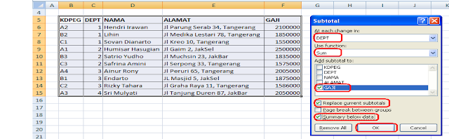

(Gambar 5. Kotak dialog Subtotals)
6. Hasil:

(Gambar 6. Hasil)
7. Untuk menghilangkan Subtotals, pada tab Data pilih icon Subtotals kembali. Akan muncul kotak dialog Subtotals dan klik Remove All

(Gambar 7. Untuk menghilangkan subtotals)
8. Untuk menyaring data dengan kriteria tertentu, posisikan kursor pada salah sel dalam tabel. Lalu pada tab Data pilih icon Filters.

(Gambar 8. Menyaring data denga criteria)
9. Pada tabel akan muncul tampilan seperti dibawah ini

(gambar 9, lihat table)
10. Misal untuk menyaring data karyawan yang lebih besar dari 1850000, maka klik pada tombol drop down di kolom GAJI, pilih Number Filters > Greater Than

(Gambar 10. Data karyawan yang disaring)
11. Akan muncul kotak dialog Custom Auto Filter, lalu isikan seperti pada gambar, klik OK

(Gambar 11. Kotak dialog Costum AutoFilter)
12. Hasil:
(Gambar 12. Hasil)
13. Untuk mengembalikan tampilan seperti semula, klik tombol drop down pada kolom GAJI pilih Clear Filter from “GAJI”. Lalu klik icon Filter pada tab data

(Gambar 13, untuk menampilkan semula)
14. Untuk menampilkan data dengan PivotTable dan PivotChart sekaligus, posisikan kursor pada salah sel dalam tabel. Lalu pada tab Insert pilih icon PivotTable, klik PivotChart

(Gambar 14. Pivottable sekaligus Pivotchart)
15. Akan muncul kotak dialog Create PivotTable with PivotChart. Pada Table/Range akan otomatis terisi dengan range tabel data. Apabila belum sesuai, bisa klik pada tanda panah lalu sorot keseluruhan tabel data. Klik OK

(Gambar 15. Data Create Pivot Table with PivotChart)
16. Pada sheet baru akan muncul tampilan seperti di bawah ini

(Gambar 16. PivotChart Filter Pane)
17. Misal kita ingin tampilkan data Nama dan Gaji masing-masing karyawan. Pada panel Pivot Table Field List beri tanda cek pada field Nama dan Gaji

(Gambar 17. PivotTable Field List)
18. Hasil

(Gambar 18, hasil)
Latihan 13 (Grafik)
Latihan 13 (Grafik)
Grafik adalah tampilan secara visual dari sebuah data. Untuk membuat grafik di Microsoft Excel 2007, data terlebih dahulu harus tersedia pada suatu worksheet.
Untuk berlatih dengan fasilitas grafik di Microsoft Excel 2007, ikuti panduan di bawah ini:
1. Buatlah tabel seperti di bawah ini, lalu sorot range A3:C10

(Gambar 19. Daftar kebutuhan Barang)
2. Pada tab Insert group Charts klik icon type grafik yang akan dipilih. Misal Pie, lalu pilih salah satu jenisnya. Untuk jenis pilihan yang lebih lengkap bisa klik All Chart Types.
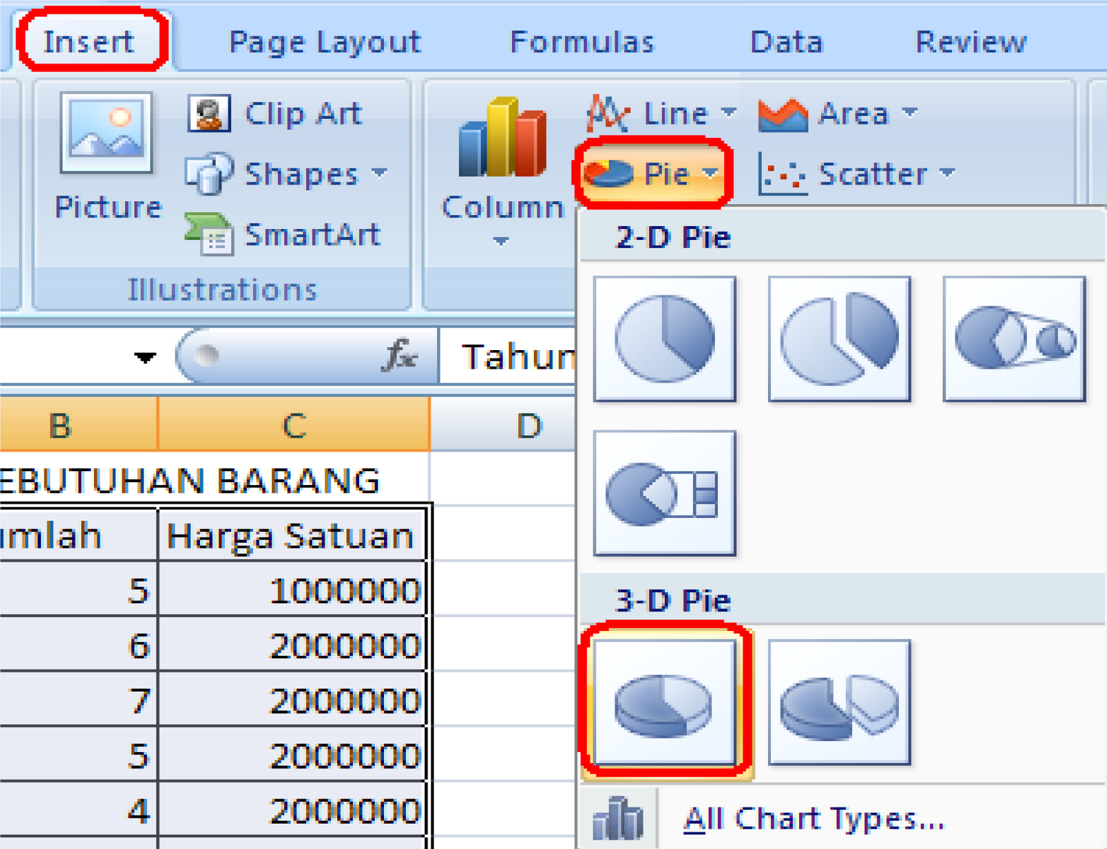
(Gambar 20. Insert Group Charts)
3. Akan muncul tampilan seperti di bawah ini. Untuk mengubah legenda klik kanan pada box legenda lalu klik Select Data

(Gambar 21. Table diagram)
4. Pada kotak dialog Select Data Source klik Edit. Akan muncul kotak dialog Axis Labels lalu sorot range A3:A10 pada tabel.

(Gambar 22. Select data Source)
5. Hasilnya seperti di bawah ini lalu klik OK. Lanjutkan klik OK pada kotak dialog Select Data Source.

(Gambar 23. Table tahun)
6. Untuk mengganti judul grafik, klik 2 kali pada judul grafik lalu ketikkan seperti di bawah ini

(Gambar 24, table kebutuhan)
7. Untuk mengubah layout grafik klik box grafik terlebih dahulu lalu pilih tab Design lalu klik icon Layout. Misal pilih Layout 2. Kecilkan ukuran grafik sesuai kebutuhan

(Gambar 25, design table)
8. Untuk menambahkan halaman dengan clipart pilih tab Insert lalu klik ClipArt. Posisikan kursor di salah sel. Akan muncul panel Clip Art lalu pilih salah satu gambar. Klik pada tombol dropdown lalu klik Insert.

(Gambar 26, insert)

(Gambar 27, clipart)
9. Kecilkan gambar dan posisikan di atas tabel sebelah kiri. Lebarkan tinggi sel A dengan cara menarik baris sel ke bawah (lihat kursor panah di antara baris 1 dan 2). Untuk variasi tampilan klik tab Format lalu pada group Picture Styles pilih icon Drop Shadow Rectangle

(Gambar 28, daftar kebutuhan barang)
10. Untuk menambahkan wordart pilih tab Insert lalu klik Icon WordArt. Pilih salah satu style wordart.

(gambar 29. Word art)
Lalu klik box wordart lalu pilih tab Home, ganti font menjadi ukuran 28. Posisikan box wordart di sebelah gambar
Lalu klik box wordart lalu pilih tab Home, ganti font menjadi ukuran 28. Posisikan box wordart di sebelah gambar

(gambar 30, klik home)
11. Lalu edit teks pada box wordart, hasilnya seperti di bawah ini

(Gambar 31, hasil selesai)
12. Selesai
IN ENGLISH (with google translate Indonesian-english)
Database in Microsoft Excel 2007
The database consists of a set of records, while the record consists of a set of fields (data) that form a single entity and each field (data) are interconnected with one another to form a certain sense.Microsoft Excel 2007 provides a variety of activities such as operation of the database sort the data, track and display the data with the filter, completing the table with a subtotal, a recapitulation of data with a pivot table, and data consolidation of multiple worksheets.
Several provisions that need to be in the makeup of the database are:
• The name field must be in one line.
• There should not be the same field name• The line directly under the title of the data considered. So do not separate the data with column headings and blank lines.
To practice with database facilities in Microsoft Excel 2007, follow the guidelines below:
Exercise 12 (Subtotals, Filters, PivotTable)
1. Create a table as below
(Table 1. Data CV employees. Komputerindo)
2. To perform data sorting is ascending by KDPEG, click any cell in column KDPEG, on the Data tab select the icon sort A to Z. To sort the data with more specific criteria can choose Sort icon.
(Table 2, how to sort the data by ascending)
3. Result
(Figure 3, the results of data)
4. To perform the summation of data per DEPT, first do the ordering data in ascending based on DEPT, by the way as in point 2.Position the cursor on any cell in the table. Then select the icon in the tab Data Subtotals
(Figure 4, the summation of data per DEPT)
5. Subtotals dialog box will appear. Follow the choice of the picture, then click OK
(Figure 5. Subtotals dialog box)
6. Results:
(Figure 6. Results)
7. To remove Subtotals, select the Data tab on the Subtotals icon back. Subtotals dialog box will appear and click the Remove All
(Figure 7. To remove subtotals)
8. To filter data by specific criteria, position the cursor on any cell in the table. Then select the Data tab on the Filters icon.
(Figure 8. Premises Data Filtering criteria)
9. On the table will appear as shown below
(Fig. 9, see table)
10. For example to filter employee data is greater than 1850000, then click on the drop down button in the column SALARY, select Number Filters> Greater Than
(Figure 10. Data employees are screened)
11. Custom dialog box will appear Auto Filter, and then fill in as shown, click OK
(Figure 11. Costum AutoFilter dialog box)
12. Results:
(Figure 12. Results)
13. To restore its original appearance, click the drop down list on the SALARY column select Clear Filter from "SALARY". Then click the Filter icon on the Data tab
(Figure 13, to display the original)
14. To display data in a PivotTable and PivotChart at once, position the cursor on any cell in the table. Then select the icon on the Insert tab PivotTable, click PivotChart
(Figure 14. PivotTable PivotChart as well)
15. Create a dialog box will appear PivotTable with PivotChart. On the Table / Range will automatically be filled with a range of data tables. If not appropriate, can click on the arrow and highlight the entire table of data. Click OK
(Figure 15. Create Pivot Table Data with PivotChart)
16. In the new sheet will appear as below
(Figure 16. PivotChart Filter Pane)
17. Suppose we want to show the data name and salary of each employee. In the Pivot Table Field List panel with checkmarks in the Name field and Salaries
(Figure 17. PivotTable Field List)
18. Result
(Figure 18, results)
Exercise 13 (Graph)
The graph is a visual display of the data. To create a chart in Microsoft Excel 2007, the data must first be available on a worksheet.To practice with chart facilities in Microsoft Excel 2007, follow the guidelines below:
1. Make a chart like this, then highlight the range A3: C10
(Figure 19. List of Goods needs)
2. Charts group on the Insert tab click the icon to be selected chart type. Eg Pie, and then select one of its kind. For a more complete kind of choice can click All Chart Types.
(Figure 20. Insert Group Charts)
3. Will appear as below. To change the legend on the right-click the legend box and click the Select Data
(Figure 21. Table diagram)
4. In the Select Data Source dialog box click Edit. Will appear Axis Labels dialog box and then highlight the range A3: A10 on the table.
(Figure 22. Select Data Source)
5. The results are shown below and then click OK. Continue to click OK on the Select Data Source dialog box.
(Figure 23. Table-year)
6. To change the chart title, click 2 times on the chart title and then type as below
(Figure 24, the table needs)
7. To change the layout of the graph click chart to first box and select the Design tab and then click the Layout icon. Eg select Layout 2. Reduce the size of the graph as needed
(Figure 25, the design table)
8. To add a page with clipart select the Insert tab and then click ClipArt. Position the cursor in any cell. Clip Art pane will appear and select a picture. Click on the dropdown button and then click Insert.
(Fig. 26, insert)
(Figure 27, clipart)
9. Shrink the image and position it above the table to the left. cellof A of high stretch by pulling down the cell lines (see the arrow cursor between lines 1 and 2). To display the variation Format tab and then click on the Picture Styles group select Drop Shadow Rectangle icon
(Figure 28, a list of items needs)
10. To add WordArt select the Insert tab and click the WordArt icon.Choose one of the WordArt style.
(Picture 29. Word art)
Then click the WordArt box and select the Home tab, change the font to a size 28. Position the WordArt box next to the image
(30 pictures, click home)
11. Then edit the text in WordArt box, the results are as below
(Figure 31, the finished result)
12. Completed
Tidak ada komentar:
Posting Komentar