Penggunaan Fungsi IF, Count IF, dan Lookup di dalam Microsoft Excell


(Gambar 13, memasukkan sel sebagai lookup value) (Gambar 14, memilih range sel sebagai table Array)
IN ENGLISH(with google translate Indonesian-English)
The use of function IF, IF Count, and Lookup in Microsoft Excell
(Source: Mr. Yudho, Computer Teach, for class XI IPS semester 2)
• 7.1 Use IF
Function IF function to complete format:
= IF (logical_test; value_if_true; calue_if_false)
Where:
1. Logical_test is suarat of branching
2. Value_if_true branching is the if condition met
3. Value_if_false is the value if the branching condition is not met
Step-by-step through the function wizard to complete the following:
1. Click on cell D3
2. Click from the menu click Insert -> Function, then this window appears, select the IF function, click OK
3. Change the setting on the window IF function as follows:
Type the text "LULUS (passed)" on the field value_if_true, which means that if the logical_test is true then this text will be produced / released.
Type the text "Tidak Lulus(Not Passed)" on the field value_if_false, which means that if the logical_test is false then this text will be produced / released.
4. Click OK. Copy the formula into the cell below it Flagging " " is an additional statement if you want to add a sentence or a string. Obtain the final result as shown below:
Ramifications not only the separation into two possibilities, but also could be a lot of possibilities. For the separate branching into many possibilities to use IF the story.
• 7.1 Branching Several Levels
= IF (OR (Logika1 Tests: Tests Logika2); Value if true: value if false)
Case study: a company will recruit security guards (guards) the following conditions: a minimum of four years of work experience and maximum age 35 years. Administration of the company doing the selection criteria, the eligible applicants will follow the next condition, while those not eligible disqualified. Case can be translated into IF function as follows:
= IF (AND (Employment> = 4; Age <= 35); Interview; Fall)
= IF (D5 <60, "E", (IF (D5 <75, "D", IF (D5 <85, "C", IF (D5 <95, "B", "A")))))
• 7.3 Finding Number
A list of values we want to know how many people who got an "A". For it provided the function: = COUNTIF (range, criteria)
Where the area specified in the range to search how many cells are in accordance with the criteria. Example = COUNTIF (B2: B57, "A") means to look for how the number of cells containing the "A" in the range B2 to B57. Example, was developed to find the Number of Passed and Failed:
• 7.4 Other functions of the Reference Lookup
Settlement may be used if the number of groups that exist only a few and will not change, what if the group reaches 100 or plus?.
Shape functions:
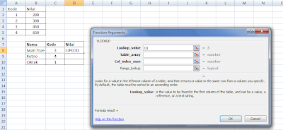
VLOOKUP (lookup value, table_array, col_index_num [, range_lookup])
And
HLOOKUP (lookup value, table_array, col_index_num [, range_lookup]) Where:
• lookup_value is data to be matched.
• table_array is where the search data.
• col_index_num keberapa column is the data on which to capture
• range_ lookup (optional) is the logic value is entered, if TRUE then filled up the data to be searched nearby, while if it is filled FALSE it will look exactly the same data.
The use VLOOKUP to the above case is in cell D8 will we enter the formula = VLOOKUP (C8, $ A $ 2: $ B $ 5.2), where C8 is the key data that will be matched, $ A $ 2: $ B $ 5 is the search area data, including search key and data to be retrieved, and the second is to show the 2nd column of the data range is taken. Or in another way by using the function wizard follows:
1. Place the cursor on cell C8
2. Click Insert-> Function
3. Select Lookup & Reference category
4. Select Menu VLOOKUP. Click OK. 5. In the Wizard select VLOOKUP menu or type in cell C8

7. Add the $ sign for the Range, so it becomes $ A $ 2: $ B $ 5, $ sign is to be the absolute cell so that if the copu to the cell below it does not change the reference. 8. Type 2 which will restore to 2 on col_index_num, for he explained:


9. Click OK, then copy it to the cell below it. The results are as shown below:

(Sumber: Mr Yudho, Computer Teach, for class XI IPS semester 2)

(Gambar 1 Data awal untuk mencari kelulusan)
Untuk mendapatkan status “LULUS”, mahasiswa harus mempunyai nilai lebih besar dari 50, sehingga jika nilainya kurang dari 50 maka akan diberi status “TIDAK LULUS”.
· 7.1 Penggunaan Fungsi IF
Fungsi IF dengan Format lengkap:
=IF(logical_test;value_if_true;calue_if_false) |
Dimana:
1. Logical_test merupakan suarat dari percabangan
2. Value_if_true merupakan nilai jika syarat percabangan terpenuhi
3. Value_if_false merupakan nilai jika syarat percabangan tidak terpenuhi
Langkah-langkah untuk menyelesaikan melalui function wizard adalah sebagai berikut:
1. Klik pada sel D3
2. Klik dari menu Klik Insert -> Function, kemudian muncul window seperti ini, pilih Fungsi IF, klik OK

(Gambar 2 Pemilihan Fungsi ID melalui Category Logical)
3. Ubah setting pada window fungsi IF seperti berikut:

(Gambar 3. Setting melalui function wizard)
Pada Logical Test ditulus C3 > 50 adalah karena di sel C3 lah letak dari nilai yang akan dilakukan penyeleksian. Ketikkan syaratnya pada isian logical_test, misalnya C3 > 50, yang artinya jika data di cell C3 lebih besar atau sama dengan 50 maka bernilai benar dan jika kurang dari 50 maka bernilai salah.
Ketikkan teks “Lulus” pada isian value_if_true, yang artinya jika pada logical_test bernilai benar maka teks ini yang akan dihasilkan/ dikeluarkan.
Ketikkan teks “Tidak Lulus” pada isian value_if_false, yang artinya jika pada logical_test bernilai salah maka teks ini yang akan dihasilkan/ dikeluarkan.
4. Klik OK. Copy-kan formula ke sel dibawahnya
Pemberian tanda “ “ merupakan tambahan jika ingin menambahkan statement berupa kalimat atau string.
Didapatkan hasil akhir seperti gambar berikut:

(Gambar 4. Hasil Akhir pemberian status kelulusan)
Fungsi | Keterangan |
IF | Menentukan suatu tes logika untuk dikerjakan, dan mempunyai bentuk: =IF(tes logika, nilai jika benar, nilai jika salah) |
AND, OR, dan NOT | Merupakan fungsi tambahan untuk mengembangkan tes kondisi. Fungsi AND dan OR maksimal berisi 30 argumen logika, sedangkan NOT hanya mempunyai satu argument logika, mempunyai bentuk: AND( logika1, logika2, …….logika30) OR(logika1, logika2, …….logika30) NOT (logika) |
Percabangan tidak hanya pemisahan menjadi dua kemungkinan saja, namun juga bisa menjadi banyak kemungkinan. Untuk percabangan yang memisahkan ke banyak kemungkinan harus menggunakan IF secara bertingkat.
· 7.1 Percabangan Beberapa Tingkat
=IF(OR(Tes Logika1;Tes Logika2); Nilai jika benar; Nilai jika salah) |
Studi kasus: sebuah perusahaan akan merekrut tenaga satuan pengaman (satpam) dengan ketentuan: pengalaman kerja minimal empat tahun dan usia maksimal 35 tahun. Perusahaan melakukan seleksi administrasi dengan criteria tersebut, pelamar yang memenuhi syarat akan mengikuti syarat selanjutnya, sedangkan yang tidak memenuhi syarat dinyatakan gugur. Kasus tersebut dapat diterjemahkan ke dalam fungsi IF seperti berikut ini:
=IF(AND(Kerja>=4; Usia<=35); Wawancara; Gugur)

(Gambar 5, Fungsi IF dengan 2 tes logika)
Istilah fungsi IF bercabang adalah kasus yang mempunyai banyak tingkat pengujian tes logika yang diselesaikan dengan fungsi IF. Sebagai contoh sebuah lembar kerja berisi hasil ujian statistic, berdasarkan nilai ujian akan dikonversikan dalam bentuk huruf dengan ketentuan sebagai berikut:

(Gambar 6, Contoh Fungsi IF bercabang)
Sel E5 diisi dengan rumus:
=IF(D5<60, “E”, (IF(D5<75, “D”, IF(D5<85, “C”, IF(D5<95, “B”, “A”)))))
· 7.3 Mencari Jumlah
Sebuah daftar nilai ingin diketahui berapa orang yang mendapat nilai “A”. Untuk itu disediakan fungsi:
=COUNTIF(range, criteria) |
Dimana pada area yang disebutkan di range akan dicari berapa jumlah sel yang sesuai dengan criteria. Contoh =COUNTIF(B2:B57, “A”) artinya dicari berapa jumlah sel yang berisi “A” pada range B2 sampai B57.
Contoh, dikembangkan untuk mencari Jumlah Lulus dan Tidak Lulus:

(Gambar7, hasil akhir penambahan Fungsi COUNTIF)
Untuk dapat menambahkan hasil tersebut, lakukan penambahan fungsi COUNTIF pada C9 melalui function wizard:

(Gambar 8, pengubahan setting fungsi COUNTIF untuk sel C9)
Sedangkan untuk mendapatkan jumlah tidak lulus, lakukan penambahan fungsi COUNTIF pada C10 melalui function wizard:

(Gambar 9, pengubahan setting fungsi COUNTIF untuk sel C10)
Nilai yang kita olah melalui Excell sebenarnya dapat dibagi menjadi dua bagian, yaitu nilai formula dan nilai acuan. Yang selama ini dijelaskan pada bab-bab sebelumnya, adalah nilai formula, dimana semua nilai yang diolah menjadi satu dengan formula yang dihitung, missal=A1*20. Angka 20 merupakan nilai formula. Sedangkan pada beberapa keadaan dimana nilai tersebut sering berubah, bisa kita gunakan nilai acuan agar tidak perlu merubah melalui formula. Untuk memudahkan menggunakan nilai acuan, Excell menyediakan fasilitas Fungsi Lookup, fungsi ini akan melihat nilai pada table lain apakah nilai yang dicocokan ada pada table tersebut, untuk kemudian diambil nilainya.
· 7.4 Fungsi Lookup Reference

(Gambar 11, Contoh Penggunaan fungsi Lookup)
Permasalahan yang akan diselesaikan adalah mengisi Gaji Pokok berdasarkan data yang ada di atasnya. Hal ini sebenarnya dapat diselesaikan dengan menggunakan percabangan IF, misalnya untuk mengisi sel D8 dapat digunakan rumus =IF(C3=1, $B$2, IF(C3=2,$B$3, IF(C3, $B$4, $B$5))).
Penyelesaian tersebut dapat digunakan jika jumlah golongan yang ada hanya sedikit dan tidak akan berubah, bagaimana jika jumlah golongan mencapai 100 atau kebih ?.
Bentuk fungsinya:
VLOOKUP(lookup value,table_array,col_index_num[,range_lookup]) |
Dan
HLOOKUP(lookup value,table_array,col_index_num[,range_lookup]) |
Dimana:
· lookup_value adalah data yang akan dicocokkan.
· table_array adalah tempat pencarian data.
· col_index_num adalah data pada kolom keberapa yang hendak diambil
· range_ lookup (optional) adalah nilai logika yang dimasukkan, jika diisi TRUE maka akan dicari sampai data terdekat, sedangkan jika diisi FALSE maka akan dicari data yang persis sama.
Pemakaian VLOOKUP untuk kasus diatas adalah pada sel D8 akan kita masukkan rumus =VLOOKUP(C8,$A$2:$B$5,2), dimana C8 adalah data kunci yang akan dicocokkan, $A$2:$B$5 adalah area pencarian data termasuk kunci pencarian dan data yang akan diambil, dan 2 adalah menunjukkan kolom ke-2 dari range tersebut adalah data yang diambil.
Atau dengan cara lain dengan menggunakan function wizard berikut:
1. Letakkan kursor pada sel C8
2. Klik Insert->Function
3. Pilih kategori Lookup & Reference

(gambar 12, fungsi Vlookup ada di kategori Lookup & Reference)
4. Pilih Menu VLOOKUP. Klik OK.
5. Pada menu VLOOKUP Wizard pilih atau ketik sel C8

6. Klik tombol Browse pada Cell Range, Blok A1 hingga B5, judul kolom tidak usah dipilih
s

s
7. Tambahkan tanda $ untuk Range, sehingga menjadi $A$2:$B$5, tanda $ ini untuk menjadi sel absolute agar jika di copu ke sel dibawahnya tidak berubah referensinya.
8. Ketik 2 dimana akan mengembalikan ke 2 pada Col_index_num, untuk jelasnya:
(Gambar 15, indeks kolom pada table array)

(Gambar 16, perubahan pada isian Vlookup melalui wizard)
9. Klik OK, kemudian Copy kan ke sel dibawahnya. Hasilnya seperti gambar berikut:
(Gambar 17, hasil akhir dan contoh pengkodean)
Sebagai pedoman dalam pemakaian VLOOKUP ini adalah kunci pencarian harus berada di kolom paling kiri dari table_array dan kunci pencarian tersebut harus dalam keadaan sudah terurut.
Pemakaian HLOOKUP sama dengan VLOOKUP, Perbedaannya hanya dalam hal penyusunan datanya, yaitu kalau VLOOKUP datanya disusun secara vertical sedangkan kalau HLOOKUP datanya disusun dengan cara horizontal.
IN ENGLISH(with google translate Indonesian-English)
The use of function IF, IF Count, and Lookup in Microsoft Excell
(Source: Mr. Yudho, Computer Teach, for class XI IPS semester 2)
(Figure 1 Preliminary data to look for graduation)
To obtain the status of "PASS", the student must have a value greater than 50, so that if the value is less than 50 will be given the status of "NOT PASS".• 7.1 Use IF
Function IF function to complete format:
= IF (logical_test; value_if_true; calue_if_false)
Where:
1. Logical_test is suarat of branching
2. Value_if_true branching is the if condition met
3. Value_if_false is the value if the branching condition is not met
Step-by-step through the function wizard to complete the following:
1. Click on cell D3
2. Click from the menu click Insert -> Function, then this window appears, select the IF function, click OK
(Figure 2 Selection Function by Category Logical ID)
3. Change the setting on the window IF function as follows:
(Figure 3. Setting through the function wizard)
In the Logical Test dropped into C3> 50 is due on cell C3 is the location of the selection will be done. Type logical_test condition on the field, such as C3> 50, which means that if the data in cell C3 is greater than or equal to 50 then it is true, and if less than 50 then it is false.Type the text "LULUS (passed)" on the field value_if_true, which means that if the logical_test is true then this text will be produced / released.
Type the text "Tidak Lulus(Not Passed)" on the field value_if_false, which means that if the logical_test is false then this text will be produced / released.
4. Click OK. Copy the formula into the cell below it Flagging " " is an additional statement if you want to add a sentence or a string. Obtain the final result as shown below:
(Figure 4. Final delivery status of graduation)
Function | Description |
IF | IF Specifies a logical test to be done, and has the form: = IF (logical test, value if true, value if false) |
AND, OR, dan NOT | AND, OR, and NOT an additional function is to develop test conditions. AND and OR functions contain a maximum of 30 logical argument, while NOT have only one logical argument, has the form: AND (logika1, logika2, ....... logika30) OR (logika1, logika2, ....... logika30) NOT (logical) |
Ramifications not only the separation into two possibilities, but also could be a lot of possibilities. For the separate branching into many possibilities to use IF the story.
• 7.1 Branching Several Levels
= IF (OR (Logika1 Tests: Tests Logika2); Value if true: value if false)
Case study: a company will recruit security guards (guards) the following conditions: a minimum of four years of work experience and maximum age 35 years. Administration of the company doing the selection criteria, the eligible applicants will follow the next condition, while those not eligible disqualified. Case can be translated into IF function as follows:
= IF (AND (Employment> = 4; Age <= 35); Interview; Fall)
(Figure 5, the IF function with the 2 test logic)
The term branched IF function is a case that has many levels of testing logic testing was completed with the IF function. For example, a spreadsheet containing the results of the test statistic, based on test scores will be converted in the form of letters with the following conditions: (Figure 6, Example branched IF Function)
Tues E5 filled with the formula:= IF (D5 <60, "E", (IF (D5 <75, "D", IF (D5 <85, "C", IF (D5 <95, "B", "A")))))
• 7.3 Finding Number
A list of values we want to know how many people who got an "A". For it provided the function: = COUNTIF (range, criteria)
Where the area specified in the range to search how many cells are in accordance with the criteria. Example = COUNTIF (B2: B57, "A") means to look for how the number of cells containing the "A" in the range B2 to B57. Example, was developed to find the Number of Passed and Failed:
(Gambar7, the final addition of COUNTIF Function)
To be able to add the results, the COUNTIF function to do the addition of C9 through the function wizard: (Figure 8, changing the setting COUNTIF function to cell C9)
Meanwhile, to get the number does not pass, do the addition of the C10 COUNTIF function through function wizard: (Figure 9, the conversion setting COUNTIF function to cell C10)
The value that we if through Excell actually may be divided into two parts, namely the formula and reference values. Which has been described in previous chapters, is the formula, where all values are processed to become one with the calculated formula, eg = A1 * 20. Number 20 is the formula. While in some circumstances in which these values change frequently, we can use the reference value in order not to change through the formula. To facilitate the use of reference values, Excel Lookup function provides the facility, this function will see the value in another table if the values are matched on the table, then its value is taken.• 7.4 Other functions of the Reference Lookup
(Figure 11, Example Using Lookup functions)
Problems to be solved is to fill the Basic Salary based on existing data on it. This can actually be solved by using the branching IF, for example, to fill the cell D8 can use the formula = IF (C3 = 1, $ B $ 2, IF (C3 = 2, $ B $ 3, IF (C3, $ B $ 4, $ B $ 5))). Settlement may be used if the number of groups that exist only a few and will not change, what if the group reaches 100 or plus?.
Shape functions:
VLOOKUP (lookup value, table_array, col_index_num [, range_lookup])
And
HLOOKUP (lookup value, table_array, col_index_num [, range_lookup]) Where:
• lookup_value is data to be matched.
• table_array is where the search data.
• col_index_num keberapa column is the data on which to capture
• range_ lookup (optional) is the logic value is entered, if TRUE then filled up the data to be searched nearby, while if it is filled FALSE it will look exactly the same data.
The use VLOOKUP to the above case is in cell D8 will we enter the formula = VLOOKUP (C8, $ A $ 2: $ B $ 5.2), where C8 is the key data that will be matched, $ A $ 2: $ B $ 5 is the search area data, including search key and data to be retrieved, and the second is to show the 2nd column of the data range is taken. Or in another way by using the function wizard follows:
1. Place the cursor on cell C8
2. Click Insert-> Function
3. Select Lookup & Reference category
(Figures 12, Vlookup function in the Lookup & Reference category)

(Figure 13, enter the cell as a lookup value)
6. Click the Browse button in the Cell Range, Block A1 to B5, the title of the column is not selected. (Figure 14, select the cell range as a table Array)
7. Add the $ sign for the Range, so it becomes $ A $ 2: $ B $ 5, $ sign is to be the absolute cell so that if the copu to the cell below it does not change the reference. 8. Type 2 which will restore to 2 on col_index_num, for he explained:
(Figure 15, the index array column in the table)
(Figure 16, changes in the field through the wizard Vlookup)
(Figure 17, the final results and examples of coding)
For guidance in the use of VLOOKUP is the search key should be in the leftmost column of table_array and the search key should be in a state already sorted. The use HLOOKUP with VLOOKUP, differ only in terms of data preparation, ie if the data is arranged in a vertical VLOOKUP whereas if HLOOKUP data compiled by the horizontal.
Tidak ada komentar:
Posting Komentar